The movement of the variable in one-sided limits as a resource for teaching differential calculus
El movimiento de la variable en límites laterales de funciones irracionales como recurso para la enseñanza del cálculo diferencial
2 Universidad Autónoma de Santo Domingo (UASD), Dominican Republic.
3 University of Camagüey Ignacio Agramonte Loynaz, Cuba.
Introduction: Understanding the movement of the variable in the concept of functional limit constitutes a challenge for students beginning the study of differential and integral calculus. This difficulty is related to the multiple meanings of mathematical infinity, which transcends the everyday notion of magnitude.
Objective: To describe the behaviour of the variable in irrational functions to develop students' skills in variable movement analysis. Additionally, to offer didactic resources that allow teachers to address lateral limits from a conceptual and procedural perspective.
Methods: A descriptive-didactic analysis was carried out by solving cases of irrational functions of the form ⁿ√g(x) (with n even and g(x) polynomial). It was complemented with a quasi-experiment involving two engineering student groups: one received explicit instruction on variable movement and the other followed a traditional approach.
Results: The group that received instruction focused on variable movement analysis outperformed the control group in all assessed items, with pass rate differences ranging from 4 to 10 percentage points, depending on the complexity of the case studied.
Conclusion: Explicit teaching of variable movement in irrational functions, supported by the use of multiple registers of semiotic representation, significantly contributes to a more solid understanding of the limit concept and reduces common procedural errors.
Introducción: La comprensión del movimiento de la variable en el concepto de límite funcional constituye un desafío para el estudio del cálculo diferencial e integral. Esto se relaciona con la multiplicidad de significados del infinito matemático, que trasciende la noción cotidiana de magnitud.
Objetivo: Describir el comportamiento de la variable en funciones irracionales para el desarrollo de habilidades de análisis del movimiento de la variable en estudiantes de ingeniería. Asimismo, ofrecer recursos didácticos que permitan a los docentes abordar los límites laterales desde una perspectiva conceptual y procedimental.
Métodos: Se realizó un análisis didáctico-descriptivo mediante la resolución de casos de funciones irracionales de la forma ⁿ√g(x) (con n par y g(x) polinómica). Se complementó con un cuasi-experimento pedagógico en dos grupos de estudiantes de ingeniería: uno recibió instrucción explícita sobre el movimiento de la variable y otro siguió un enfoque tradicional.
Resultados: El grupo que recibió la instrucción focalizada en el análisis del movimiento de la variable obtuvo un rendimiento superior en todos los ítems evaluados, con diferencias porcentuales de aprobación que oscilaron entre 4 y 10 puntos respecto al grupo control.
Conclusión: La enseñanza explícita del movimiento de la variable en funciones irracionales, apoyada en el uso de múltiples registros de representación semiótica, contribuye a una comprensión del concepto de límite y reduce los errores procedimentales comunes.
Introduction
Mastering the concept of functional limit, both at an operational and conceptual level, is essential for engineering students, as it lays the foundations for differential and integral calculus (Báez & Blanco, 2020). Its study allows us to understand the various movements of the variables in relation to the concept of mathematical infinity, which is not limited to the very large, but also encompasses closeness and smallness (Mosquera-López et al., 2023).
In traditional teaching, lateral limits are mainly analyzed to verify the existence of the limit at a point. Relatively frequently the procedure consists of matching both lateral limits to guarantee the existence of the limit at the point, which is undeniably important. However, less attention is paid to the movement of the variable in irrational functions that, unlike functions defined in the entire environment, only have one of the lateral limits at certain points.
To theoretically substantiate the proposal, the contributions of Duval (2004) on the need for conversion between semiotic registers (algebraic, graphic and numerical) are articulated with the distinction between conceptual and procedural knowledge proposed by Rittle-Johnson and Koedinger (2009). Along these lines, it is documented that errors in lateral limits usually originate from a static interpretation of infinity and the predominance of algebraic treatment over the analysis of the domain and the sign of the function. The absence of systematic work with conversions between registers prevents students from perceiving the behavior of the variable in the vicinity of the critical point (Guarin Amorocho & Parada Rico, 2023).
This omission makes the concept difficult to understand; as a result, students often make mistakes when analyzing these cases in a simplistic way. For example, in the function f(x) = √(x − 2), when computing the limit of the function f(x) when x → 2 they generally ignore the discontinuity at x = 2, and attempt a direct evaluation that leads to limx→2 √(x − 2) = √(2 − 2) = 0. This result –strictly speaking– is incorrect, because the left limit does not exist since its expression is not defined in real numbers.
Errors like this show inefficient prior training, in which the need to analyze the domain and path of a function before operating with it is not sufficiently emphasized (Byas & Blanco, 2017). This problem is linked to the student's procedural knowledge, since the final result is often prioritized without paying sufficient attention to the details of the process (Rittle-Johnson & Koedinger, 2009).
Taking the above into account, it is postulated that excessive attention to algebraic complexity in limit exercises can divert the focus from conceptual understanding. For this reason, this article aims to describe the behavior of the variable in irrational functions for the development of variable motion analysis skills in engineering students. Likewise, it is intended to offer teaching resources that allow teachers to address lateral limits from a conceptual and procedural perspective.
Methods
The study was carried out in two complementary phases. The first phase, of a theoretical nature, consisted of a rigorous mathematical analysis of the algebraic structure of irrational functions of the form ⁿ√g(x), where n is even, g(x) is a polynomial function and g(c) = 0. The purpose of this phase was to characterize the behavior of the lateral limits at points where the subradical expression is nullified. This analysis –which started from the study of particular cases– allowed us to build a systematic classification of three general cases based on the nature of the root c of g(x): simple root, root of odd multiplicity and root of even multiplicity. This result was transformed into an explicit teaching resource for teaching the concept of lateral limit.
The second phase, empirical in nature, adopted a quasi-experimental design with two parallel groups of engineering students (Group A and Group B), both attended by professors of similar experience. Its objective was to evaluate the effectiveness of the teaching resource on student performance when solving problems of lateral limits in irrational functions.
Participants and context
For the quasi-experiment, the sample was made up of 79 first-year engineering students from the Autonomous University of Santo Domingo (Dominican Republic), distributed into two natural groups: Group A (experimental, n = 38) and Group B (control, n = 41). The average age was 19.2 years (SD = 1.4) and 62 % were male. All had passed a precalculus course with similar average grades (Group A: 72.4 out of 100; Group B: 71.9). They come from public (65 %) and private (35 %) educational centers, with a predominance of public schools. Both groups shared the same curriculum and had previously studied the same basic mathematics content.
Procedure
The quasi-experiment adopted a classical research structure. It consisted of the application of an entry diagnostic test (pretest), followed by a pedagogical intervention and closed with the application of a final diagnosis, also known as postest.
Pretest
The pretest contained five exercises that required analyzing the domain of an irrational function with an even index and determining the existence of lateral limits at points where the radicand cancels out. The items included concrete examples such as: analyze the domain of f(x) = √(x − 2) and determine if limx→2 √(x − 2) exists; study the behavior of g(x) = ∛(x − 2) in the vicinity of x = 2; and explore cases with roots of even multiplicity such as √(−(x − 2)²).
Special attention was paid to students justifying the existence or not of the limit based on the sign of the radical and not only through algebraic manipulation. The results were compared with a Student t test for independent samples, which did not yield statistically significant differences (t = 0.42; df = 77, p = 0.68). Likewise, the Mann-Whitney U test was applied as a non-parametric contrast, obtaining U = 756.5 (p = 0.72), which confirms the initial homogeneity of the groups in terms of prior knowledge about the object of study. This equivalence made it possible to attribute post-intervention differences.
Didactic intervention
In Group A (experimental), two class sessions of 90 minutes each (total 3 hours) were dedicated to the explicit analysis of cases of movement of the variable in irrational functions. The intervention included specifically designed materials:
- Work guide structured in three columns: (1) algebraic expression of f(x), (2) table of signs of the radicand g(x), (3) graphic sketch of f(x) and determination of lateral limits.
- Guided presentation of the three theoretical cases (simple root, root of odd multiplicity, root of even multiplicity) with the support of graphic representations prepared in GeoGebra.
- Conversion activities between registers: the analytical expression of f(x) was provided and students were asked to construct the sign table, sketch the graph, and decide the existence of the limit.
- Collective discussion of typical errors, such as direct evaluation without considering the sign of the radicand.
In Group B (control) teaching was developed in a traditional way, following the usual textbook, with emphasis on algebraic manipulation and direct evaluation of limits. Algebraic simplification and on-point evaluation were worked on, without emphasizing the systematic analysis of the domain and the movement of the variable.
To avoid bias, the same teachers taught both modalities; standardized teaching guides were designed and a prior meeting was held to agree on the contents and duration, ensuring that the only difference was the focus on the movement of the variable and the use of multiple registers. The verification test was administered one week after the intervention to allow the content to be consolidated and avoid the effect of short-term memory, without additional directed practice between both dates.
Verification instrument (postest)
The dependent variable was performance in solving boundary problems, measured by a verification test administered at the end of the teaching unit (one week after the intervention). The instrument evaluated the following types of exercises:
- Analyze the limits of the function at x = 2, x = -2.
- Analyze the limits of the function at x = 1.
- Analyze the following limits at the indicated point:
- 3.1) limx→γ (ln(sin(x))·sin(x))
- 3.2) limx→γ ln(sin(x))/cos(x)
- 3.3) limx→γ ln(sin(x))/cos(x)
Each item was graded as approved if the student correctly justified the existence or not of the lateral limits through the analysis of the sign of the radical and the domain of the function, without being limited to direct evaluation. Partial credit was awarded if the student identified the correct result but did not adequately justify the reasoning.
Statistic Analysis
To compare the results of the post-test, the Student t test for independent samples was applied to each item, after verification of normality (Shapiro-Wilk) and homogeneity of variances (Levene). Since some distributions did not meet the assumption of normality, it was complemented with the Mann-Whitney U test. The effect size was calculated using Cohen's d for each item, interpreting it according to the conventional criteria (Cohen, 1988): small (0.2), medium (0.5) and large (0.8). The level of significance was set at α = 0.05. Analyzes were performed using SPSS version 25 software.
Ethical considerations
The study was approved by the Ethics Committee of the Autonomous University of Santo Domingo. All participating students signed an informed consent in which the purpose of the research, the confidentiality of the data, and their right to withdraw at any time were explained. The results obtained were only used for research purposes.
Results and discussion
I. Characterization of the behavior of the lateral limits at points where the subradical expression is nullified
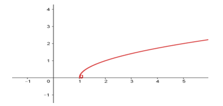
The analysis of particular cases allowed us to take a first example for theoretical argumentation; this is the function f(x) = √(x − 1), which presents a difficulty for students who have not been trained in case analysis. Here the lack of precision of the movement of the variable leads many students not to pay attention to the fact that if x < 1 the subradical quantity is negative and therefore the domain of the function is only for x ≥ 1, as shown in Figure 1:
To a large extent this is due to the little use of changes in the semiotic representation of mathematical objects. The specialized literature abounds in works explaining the need to use different representation registers so that students can appreciate the different characteristics of the object studied (Báez & Blanco, 2020; Elia & Spyrou, 2006) given that it is very unlikely that a specific representation shows all the characteristics of the object studied.
In the case of the function f(x) = √(x² − 4x + 4), whose graph (Figure 2) shows that it is a function defined throughout its domain, from the analytical representation the domain and range of the function are not immediate, but from its graphic representation these aspects of the function are immediate:
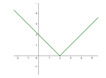
Therefore, the analysis of limx→2 √(x² − 4x + 4) is simplified because from the graph it can be seen that the variable approaches 2 in the same way from the right as from the left; that is, the variable moves to the point in the same way from the right as from the left, so the limit value can be obtained by direct evaluation. Of course this analysis can also be done analytically, but it is appropriate to show students different resources.
Analytically we have: √(x² − 4x + 4) = √((x − 2)²) = |x − 2|, where it is easily seen that it is a function with domain and range in all real numbers.
A third case is now considered: Calculate limx→2 √(−x² + 4x − 4), again in this case the student considers that they can directly evaluate and obtain:
The radicand function g(x) = −x² + 4x − 4 is a parabola with vertex at (2, 0), but since the coefficient of x² is negative the parabola opens downward (toward negative values), so it is the only real value of the radicand; since there are no lateral limits, therefore the limit at the point does not exist. This analysis can be corroborated with the graphic representation of g(x) = −x² + 4x − 4 (Figure 3):
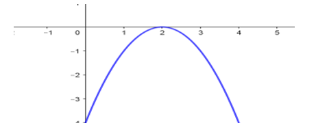
The fact that the same thing happens on both sides of the point and, despite that, the limit does not exist, creates some doubt in the student regarding his conception that the limit does not exist at the point when there are different values on both sides of the point. For this reason, we must return to the definition of limit:
Let f be a function defined in a neighborhood of point b. It is said that limx→b f(x) = L, if for each positive number ε > 0, no matter how small, it is possible to determine a positive number δ > 0, such that for all values of x, different from b, that satisfy the inequality |x − b| < δ, the inequality |f(x) − L| < ε is verified.
As you can see in this case there is no value of x in the interval |x − b| < δ so it can be stated that there is no limit in (2, 0). Here it should be noted that mathematical objects, since they do not have physical existence, are rigorously determined by their definition (Báez & Blanco, 2020; Byas & Blanco, 2017).
Based on the previous examples, some general clarifications can be made to guide students in working with this type of functions of the form: limx→c ⁿ√g(x), when n is even, g(x) is a polynomial function and g(c) = 0.
Case 1: if c is the simple root of g(x) which implies that g(c) = 0 and g'(c) ≠ 0 then limx→c ⁿ√g(x) never exists.
Justification: If c is the simple root of g(x) then there is a change of signs for values around c, which implies that one of the lateral limits does not exist.
The following graphic support (Figure 4) is important here:
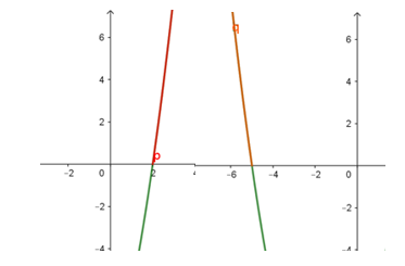
In the first graph you can see that the values to the left of 2 are negative and in the second the values to the right of -5 are negative. Therefore, for the given conditions and the root is simple, there is no limit at the point.
To explain why the limit does not exist in the case analyzed, the need to use different semiotic representations is appreciated so that students can appreciate different aspects of the object studied, specifically the movement of the variable (Elia & Spyrou, 2006).
Case 2: if c is the root of odd multiplicity of g(x) then limx→c ⁿ√g(x), never exists.
A root of odd multiplicity implies a cut of the graph of g on the x axis where the concavity changes; that is, if c is a root of odd multiplicity of g, it is also an inflection point of g, which determines a change of sign for values close to c, so one of the lateral limits does not exist. Graphic support is also very useful here (Figure 5) so that students can materialize the previous explanation through the semiotic materialization of the mathematical object (Rodríguez & López Fernández, 2010):
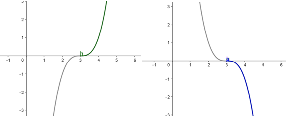
In this example c = 3 is a point where the concavity changes, so in the first case the lateral limit does not exist for values less than 3 and in the second it does not exist for values greater than 3.
At this point it is appropriate to insist to students on the need to keep in mind the conditions of the problem with which they are working, since the fact that the function has a negative branch around the point being analyzed does not prevent verifying the relationship, but it cannot be forgotten that the function being considered is a subradical quantity in a root of even index, so the root does not exist for negative values of g(x). This clarification may seem unimportant but it is made with the aim of reminding students of the need to keep in mind the hypotheses of the problem with which they are working.
Case 3: if c is a root of even multiplicity of g(x), then limx→c g(x) may or may not exist; the following cases are analyzed below:
3.1) if g is of degree 2 and the principal coefficient is greater than zero, then limx→c g(x) = 0 exists, since g is a parabola with vertex on the x axis that opens upward (this case has already been analyzed), which implies that g(x) is greater than zero for its entire domain.
3.2) if g is of degree 2 and the principal coefficient is less than zero, the parabola has its vertex on the x axis but opens downward, since g(x) is less than zero for all values of its domain and therefore √g(x) does not exist, so we cannot speak of a real limit for an expression that does not exist in ℝ.
3.3) if g is a polynomial of degree 3, in this case several alternatives arise, but when it has only a simple root the analysis coincides with the cases previously analyzed. Therefore, attention will be devoted to cases in which the polynomial has three roots, which gives rise to different situations.
In polynomials of degree 3, one branch opens upwards (looking for positive values) and another downwards (looking for negative values). Furthermore, by the fundamental theorem of algebra, a polynomial of degree 3 has 3 real or complex roots. Even complex roots appear in pairs, each root with its conjugate; therefore, if the polynomial is of degree 3 and has a double root it will also have a simple one.
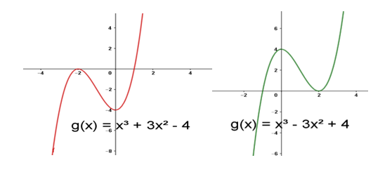
On the other hand, when the principal coefficient is positive, the left side opens toward negative values and the right toward positive ones. Therefore, if the double root is less than the simple root, the values of the function around it are negative and, around the simple root they will be negative to the left and positive to the right of the root, so in this case the limit does not exist.
But, if the simple root is less than the double root, the function will have positive and negative values around the simple root, so the limit will not exist on this root. But around the double root it will have positive values, so the limit will exist on this root, as illustrated (Figure 6) below:
On the other hand, when the coefficient of the variable with the highest degree (principal coefficient) is negative, then the left branch grows by positive values and the right branch by negative values. Therefore: if the double root is less than the simple root, the limit will exist in the double root, but not in the simple root. If the simple root is smaller, the limit will not exist in either of the two roots, as illustrated in Figure 7:
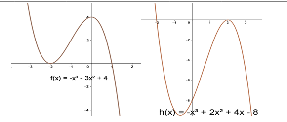
Keep in mind that we are talking about the values in the subradical function, so when this function takes negative values it is not defined in the real values and the limit cannot exist.
This analysis is applicable to any polynomial radicand of the form g(x) = anxn + an−1xn−1 + … + a0 with an ≠ 0, taking into account:
- The roots of even multiplicity of g(x)
- The simple or odd multiplicity roots of g(x)
- The sign of the leading coefficient an
- The relative position of each multiple root with respect to the other roots
In general, the activity of considering different representations of a mathematical concept is not considered fundamental by many teachers for the construction of said concept. In particular, activities that involve conversion-type and treatment-type transformations (Duval, 2004) are minimized by teachers when studying the functions, unaware that they promote a better understanding of the functions and facilitate the development of visualization processes (Amaya De Armas et al., 2016).
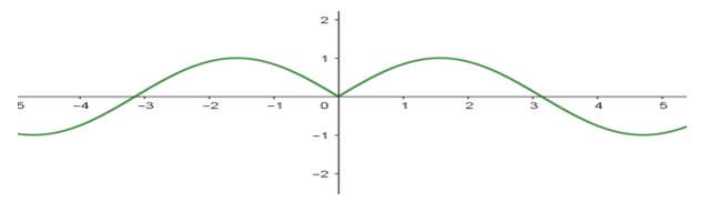
From a didactic perspective, the analysis of the calculation of limits in different cases –in this type of functions– is not done only with the objective of training the student in this specific topic. Procedural work provides training to students that improves their understanding of the behavior of the limit of functions, in particular the implications of lateral limits on the existence of the limit of a function. For example, in the case limx→0 x/|x| students better understand that the given limit does not exist, that on the left the variable approaches zero for negative values and, on the right, for positive values.
However, in the case limx→0 x·sin(x)/|x| = 0 it can be seen that the numerator is the product of two odd functions, therefore, it is even. The denominator is even; therefore, the function is even, so its behavior is the same to the left and right of the x axis. In other words, the variable moves in the same way on both sides of the point as can be seen in Figure 8:
II. Results of the didactic intervention
| Item | Group A (experimental, n = 38) | Group B (control, n = 41) | ||
|---|---|---|---|---|
| Approved | % | Approved | % | |
| 1 | 27 | 71.05 | 26 | 63.41 |
| 2 | 28 | 73.68 | 26 | 63.41 |
| 3.1 | 23 | 60.53 | 23 | 56.10 |
| 3.2 | 22 | 57.89 | 22 | 53.66 |
| 3.3 | 22 | 57.89 | 21 | 51.22 |
Table 1 shows that Group A (experimental) outperformed Group B (control) on all items. The percentage differences in approval were: 7.64 points in item 1; 10.27 points in item 2; 4.43 points in 3.1; 4.23 points in 3.2 and 6.67 points in 3.3.
These results reflect that the explicit teaching of the cases of movement of the variable and the use of different registers of semiotic representation especially benefited the resolution of the exercises with a simple root (items 1 and 2). In them, the most frequent error of the control group was to carry out a direct evaluation ignoring that one of the lateral limits does not exist because the radical takes negative values. The experimental group, on the other hand, showed greater ability to examine the domain and sign of the radical before operating, which led to a larger difference.
In items 3.1, 3.2 and 3.3, corresponding to roots of even multiplicity with various sign configurations, the advantage of the experimental group persisted but was more modest. The approval rate in both groups was lower than in the previous items, indicating that these cases represent a greater cognitive challenge. To solve them correctly, the student must integrate the analysis of the multiplicity of the root, the sign of the principal coefficient and the relative position of the roots, transforming the algebraic information into a graphical representation or into a judgment about the existence of the limit.
Explicit instruction helped a greater proportion of students in Group A to coordinate these criteria, but the smaller difference suggests that consolidating this reasoning requires more practice time and a deeper internalization of representational transformations. Table 2 shows the descriptive statistics and the results of the parametric and non-parametric tests and the effect size.
| Item | Group A (experimental, n = 38) | Group B (control, n = 41) | t (df = 77) | p (t) | U | p (U) | Cohen's da | ||
|---|---|---|---|---|---|---|---|---|---|
| Mean | Standard Deviation | Mean | Standard Deviation | ||||||
| 1 | 7.42 | 2.10 | 6.05 | 2.45 | 2.68 | 0.009 * | 545 | 0.011 * | 0.62 |
| 2 | 7.68 | 1.95 | 6.22 | 2.30 | 3.04 | 0.003 * | 512 | 0.005 * | 0.69 |
| 3.1 | 6.05 | 2.80 | 5.51 | 2.75 | 0.87 | 0.387 | 700 | 0.392 | 0.20 |
| 3.2 | 5.89 | 2.95 | 5.32 | 2.85 | 0.86 | 0.392 | 711 | 0.421 | 0.19 |
| 3.3 | 5.97 | 2.88 | 5.15 | 2.92 | 1.26 | 0.211 | 660 | 0.184 | 0.28 |
The results in Table 2 indicate that the differences are statistically significant only for items 1 and 2 (p < 0.05 in both tests), with medium effect sizes (d = 0.62 and 0.69 respectively), indicating a practically relevant magnitude. For items 3.1 to 3.3 statistical significance is not reached (p > 0.05) and the effect sizes are small (d < 0.3), although a trend favorable to the experimental group is maintained.
To interpret the non-significant differences in items 3.1–3.3, cognitive load theory (Sweller, 1988) is useful, since these items require coordinating multiple criteria (multiplicity, sign, relative position), which can saturate students' working memory, especially in limited instruction time. These findings coincide with those reported by Guarin Amorocho and Parada Rico (2023), who point out that a deep understanding of the limit requires a fluid transition between the algebraic and the geometric, as well as sufficient time for the assimilation of the different registers of representation.
Altogether, the findings confirm that the didactic proposal contributes to reducing the direct evaluation error and strengthening the conceptual understanding of the limit, especially when the complexity of the subradical function is moderate. The observed differences correspond directly to the theoretical cases systematized in the first phase of the study.
Conclusions
The theoretical analysis made it possible to classify the lateral limits of irrational functions in three cases according to the nature of the radical root: simple root, root of odd multiplicity and root of even multiplicity. This classification constitutes a didactic resource that explains the need to analyze the domain and the sign of the radicand before operating.
The didactic intervention, which emphasized the movement of the variable supported by multiple registers of semiotic representation, produced improvements in the performance of the experimental group in all the items evaluated. The most notable difference was observed in the basic exercises, with medium effect sizes, where the direct evaluation error was smaller. In the cases of greater complexity (even multiplicity root with different sign configurations), the advantage persisted but was more modest, suggesting that a deep understanding of these cases requires longer work and finer integration between the algebraic and graphic registers.
The results confirm that the explicit teaching of the prior analysis of the domain and the behavior of the variable, as opposed to a purely procedural approach, contributes to reducing frequent conceptual errors and favors a more solid understanding of the concept of limit. Furthermore, the fundamental role of representation transformations (conversion and treatment) is evident for students to perceive the behavior of the function in environments where the analytical expression is opaque.
Limitations of the study are identified that must be considered: the use of groups (non-randomized) limits the generalization of the findings; the specific context (University of the Dominican Republic) may not be representative of other populations; and the measurement was carried out in the short term (one week after the intervention), so long-term retention or transfer to other calculation contents was not evaluated.
It is recommended that teachers dedicate at least two class sessions to the analysis of cases of simple roots and odd multiplicity, before addressing cases of even multiplicity, and to include conversion exercises between algebraic and graphical representations from the beginning of the course. It is also suggested to extend the practice time in the most complex cases and use dynamic visualization tools (GeoGebra, Matlab) to facilitate the exploration of the movement of the variable. Future research should examine the long-term retention of this learning and its transfer to other content, as well as replicate the study with more robust experimental designs (random assignment) and larger and more diverse samples.
References
- Amaya De Armas, T. R., Pino-Fan, L. R., & Medina Rivilla, A. (2016). Evaluación del conocimiento de futuros profesores de matemáticas sobre las transformaciones de las representaciones de una función. Educación Matemática, 28(3), 111-144. https://doi.org/10.24844/em2803.05
- Báez Ureña, N., & Blanco Sánchez, R. (2020). La epistemología de la matemática en su didáctica. Mikarimin. Revista Científica Multidisciplinaria, 6(3), 105-116. https://revista.uniandes.edu.ec/ojs/index.php/mikarimin/article/view/2057
- Byas, R., & Blanco, R. (2017). Didáctica de la Matemática en la formación docente. SEDUCA. Sistema Editorial Universitario Centroamericano.
- Cohen, J. (1988). Statistical Power Analysis for the Behavioral Sciences (2nd ed.). Lawrence Erlbaum Associates.
- Duval, R. (2004). Semiosis y pensamiento humano: Registros semióticos y aprendizajes intelectuales. Universidad del Valle.
- Elia, I. & Spyrou, P. (2006). How students conceive function: A triarchic conceptual-semiotic model of the understanding of a complex concept. The Mathematics Enthusiast, 3(2), 256-272. https://doi.org/10.54870/1551-3440.1049
- Guarin Amorocho, S. A. & Parada Rico, S. E. (2023). Acciones y expresiones de la comprensión del límite de una función en un punto, por estudiantes de cálculo diferencial. Educación Matemática, 35(1), 197-223. https://doi.org/10.24844/EM3501.08
- Mosquera-López, S., Soto-Agreda, O. F., & Marmolejo-Avenia, G. A. (2023). El conocimiento acerca de las ideas matemáticas sobre el infinito: El caso de los educadores matemáticos en formación de la Universidad de Nariño. Revista Perspectivas, 8(S1), 97-103. https://doi.org/10.22463/25909215.4062
- Rittle-Johnson, B., & Koedinger, K. (2009). Iterating between lessons on concepts and procedures can improve mathematics knowledge. British Journal of Educational Psychology, 79(3), 483-500. https://doi.org/10.1348/000709908X398106
- Rodríguez, O. H., & López Fernández, J. M. (2010). A semiotic reflection on the didactics of the chain rule. The Mathematics Enthusiast, 7(2&3), 321-332. https://doi.org/10.54870/1551-3440.1183
- Sweller, J. (1988). Cognitive load during problem solving: Effects on learning. Cognitive Science, 12(2), 257-285. https://doi.org/10.1207/s15516709cog1202_4
Conflict of interests:
The authors declare that they have no conflicts of interest that affect the results or their interpretations.
Curricular synthesis:
Neel Báez Ureña. Doctor in Pedagogical Sciences. Master in Pure Mathematics. Professor of the Department of Mathematics at the Universidad Acción Pro Educación y Cultura (APEC) of the Dominican Republic.
Elizabeth Rincón Santana. Doctor in Pedagogical Sciences. Master in Mathematics. Full Professor of the Department of Mathematics of the Autonomous University of Santo Domingo.
Ramón Blanco Sánchez. Doctor in Pedagogical Sciences. Graduate in Mathematics. Full Professor and Consultant. He holds the Pablo Miquel Award and several awards from the Cuban Academy of Sciences.
Marines Angeris Artiles. Master in Mathematics Teaching. Assistant Professor of the Department of Mathematics of the Faculty of Computer Science and Exact Sciences of the University of Camagüey. She is the Head of Mathematics Education Career.
Declaration of author's responsibility:
Neel Báez Ureña and Elizabeth Rincón Santana. They carried out the systematization and assessment of the information, the execution of the research, and its writing.
Ramón Blanco Sánchez. He was in charge of the methodological direction of the research and the orientation of the pedagogical and didactic approach.
Marines Angeris Artiles. She contributed to the improvement of the scientific text. Worked on data curation and information processing and interpretation.
Edited by: Dr. C. Arnaldo Espindola Artola, Translated by: B.A. Augusto García Blanca
This is an Open Access article distributed under the terms of the Creative Commons License:
https://creativecommons.org/licenses/by-nc/4.0/deed.es_ES
which allows the unrestricted non-commercial use, distribution and reproduction in any medium, provided that the primary source of publication is properly cited.